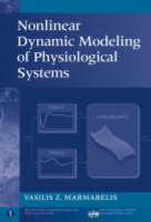
Nonlinear Dynamic Modeling of Physiological Systems
 -15%
portes grátis
Nonlinear Dynamic Modeling of Physiological Systems
Marmarelis, Professor Vasilis Z.
John Wiley & Sons Inc
09/2004
560
Dura
Inglês
9780471469605
15 a 20 dias
1186
1 Introduction 1
1.1 Purpose of this Book 1
1.2 Advocated Approach 4
1.3 The Problem of System Modeling in Physiology 6
1.3.1 Model Specification and Estimation 10
1.3.2 Nonlinearity and Nonstationarity 12
1.3.3 Definition of the Modeling Problem 13
1.4 Types of Nonlinear Models of Physiological Systems 13
Example 1.1. Vertebrate Retina 15
Example 1.2. Invertebrate Photoreceptor 18
Example 1.3. Volterra analysis of Riccati Equation 19
Example 1.4. Glucose-Insulin Minimal Model 21
Example 1.5. Cerebral Autoregulation 22
1.5 Deductive and Inductive Modeling 24
Historical Note #1: Hippocratic and Galenic Views of 26
Integrative Physiology
2 Nonparametric Modeling 29
2.1 Volterra Models 31
2.1.1 Examples of Volterra Models 37
Example 2.1. Static Nonlinear System 37
Example 2.2. L-N Cascade System 38
Example 2.3. L-N-M "Sandwich" System 39
Example 2.4. Riccati System 40
2.1.2 Operational Meaning of the Volterra Kernels 41
Impulsive Inputs 42
Sinusoidal Inputs 43
Remarks on the Meaning of Volterra Kernels 45
2.1.3 Frequency-Domain Representation of the Volterra Models 45
2.1.4 Discrete-Time Volterra Models 47
2.1.5 Estimation of Volterra Kernels 49
Specialized Test Inputs 50
Arbitrary Inputs 52
Fast Exact Orthogonalization and Parallel-Cascade Methods 55
Iterative Cost-Minimization Methods for Non-Gaussian 55
Residuals
2.2 Wiener Models 57
2.2.1 Relation between Volterra and Wiener Models 60
The Wiener Class of Systems 62
Examples of Wiener Models 63
Comparison of Volterra/Wiener Model Predictions 64
2.2.2 Wiener Approach to Kernel Estimation 67
2.2.3 The Cross-Correlation Technique for Wiener Kernel Estimation 72
Estimation of h0 73
Estimation of h1 (𝜏) 73
Estimation of h2 (𝜏1, 𝜏2) 74
Estimation of h3 (𝜏1, 𝜏2, 𝜏3) 75
Some Practical Considerations 77
Illustrative Example 78
Frequency-Domain Estimation of Wiener Kernels 78
2.2.4 Quasiwhite Test Inputs 80
CSRS and Volterra Kernels 84
The Diagonal Estimability Problem 85
An Analytical Example 86
Comparison of Model Prediction Errors 88
Discrete-Time Representation of the CSRS Functional Series 89
Pseudorandom Signals Based on m-Sequences 89
Comparative Use of GWN, PRS, and CSRS 92
2.2.5 Apparent Transfer Function and Coherence Measurements 93
Example 2.5. L-N Cascade System 96
Example 2.6. Quadratic Volterra System 97
Example 2.7. Nonwhite Gaussian Inputs 98
Example 2.8. Duffing System 98
Concluding Remarks 99
2.3 Efficient Volterra Kernel Estimation 100
2.3.1 Volterra Kernel Expansions 101
Model Order Determination 104
2.3.2 The Laguerre Expansion Technique 107
Illustrative Examples 112
2.3.3 High-Order Volterra Modeling with Equivalent Networks 122
2.4 Analysis of Estimation Errors 125
2.4.1 Sources of Estimation Errors 125
2.4.2 Estimation Errors Associated with the Cross-Correlation 127
Technique Estimation Bias 128
Estimation Variance 130
Optimization of Input Parameters 131
Noise Effects 134
Erroneous Scaling of Kernel Estimates 136
2.4.3 Estimation Errors Associated with Direct Inversion Methods 137
2.4.4 Estimation Errors Associated with Iterative 139
Cost-Minimization Methods Historical Note #2: Vito Volterra and Norbert Wiener 140
3 Parametric Modeling 145
3.1 Basic Parametric Model Forms and Estimation Procedures 146
3.1.1 The Nonlinear Case 150
3.1.2 The Nonstationary Case 152
3.2 Volterra Kernels of Nonlinear Differential Equations 153
Example 3.1. The Riccati Equation 157
3.2.1 Apparent Transfer Functions of Linearized Models 158
Example 3.2. Illustrative Example 160
3.2.2 Nonlinear Parametric Models with Intermodulation 161
3.3 Discrete-Time Volterra Kernels of NARMAX Models 164
3.4 From Volterra Kernel Measurements to Parametric Models 167
Example 3.3. Illustrative Example 169
3.5 Equivalence Between Continuous and Discrete Parametric Models 171
Example 3.4. Illustrative Example 175
3.5.1 Modular Representation 177
4 Modular and Connectionist Modeling 179
4.1 Modular Form of Nonparametric Models 179
4.1.1 Principal Dynamic Modes 180
Illustrative Examples 186
4.1.2 Volterra Models of System Cascades 191
The L-N-M, L-N, and N-M Cascades 194
4.1.3 Volterra Models of Systems with Lateral Branches 198
4.1.4 Volterra Models of Systems with Feedback Branches 200
4.1.5 Nonlinear Feedback Described by Differential Equations 202
Example 1. Cubic Feedback Systems 204
Example 2. Sigmoid Feedback Systems 209
Example 3. Positive Nonlinear Feedback 213
Example 4. Second-Order Kernels of Nonlinear 215
Feedback Systems Nonlinear Feedback in Sensory Systems 216
Concluding Remarks on Nonlinear Feedback 220
4.2 Connectionist Models 223
4.2.1 Equivalence between Connectionist and Volterra Models 223
Relation with PDM Modeling 230
Illustrative Examples 232
4.2.2 Volterra-Equivalent Network Architectures for Nonlinear 235
System Modeling Equivalence with Volterra Kernels/Models 238
Selection of the Structural Parameters of the VEN Model 238
Convergence and Accuracy of the Training Procedure 240
The Pseudomode-Peeling Method 244
Nonlinear Autoregressive Modeling (Open-Loop) 246
4.3 The Laguerre-Volterra Network 246
Illustrative Example of LVN Modeling 249
Modeling Systems with Fast and Slow Dynamic (LVN-2) 251
Illustrative Examples of LVN-2 Modeling 255
4.4 The VWM Model 260
5 A Practitioner's Guide 265
5.1 Practical Considerations and Experimental Requirements 265
5.1.1 System Characteristics 266
System Bandwidth 266
System Memory 267
System Dynamic Range 267
System Linearity 268
System Stationarity 268
System Ergodicity 268
5.1.2 Input Characteristics 269
5.1.3 Experimental Characteristics 270
5.2 Preliminary Tests and Data Preparation 272
5.2.1 Test for System Bandwidth 272
5.2.2 Test for System Memory 272
5.2.3 Test for System Stationarity and Ergodicity 273
5.2.4 Test for System Linearity 274
5.2.5 Data Preparation 275
5.3 Model Specification and Estimation 276
5.3.1 The MDV Modeling Methodology 277
5.3.2 The VEN/VWM Modeling Methodology 278
5.4 Model Validation and Interpretation 279
5.4.1 Model Validation 279
5.4.2 Model Interpretation 281
Interpretation of Volterra Kernels 281
Interpretation of the PDM Model 282
5.5 Outline of Step-by-Step Procedure 283
5.5.1 Elaboration of the Key Step # 5 284
6 Selected Applications 285
6.1 Neurosensory Systems 286
6.1.1 Vertebrate Retina 287
6.1.2 Invertebrate Retina 396
6.1.3 Auditory Nerve Fibers 302
6.1.4 Spider Mechanoreceptor 307
6.2 Cardiovascular System 320
6.3 Renal System 333
6.4 Metabolic-Endocrine System 342
7 Modeling of Multiinput/Multioutput Systems 359
7.1 The Two-Input Case 360
7.1.1 The Two-Input Cross-Correlation Technique 362
7.1.2 The Two-Input Kernel-Expansion Technique 362
7.1.3 Volterra-Equivalent Network Models with Two Inputs 364
Illustrative Example 366
7.2 Applications of Two-Input Modeling to Physiological Systems 369
7.2.1 Motion Detection in the Invertebrate Retina 369
7.2.2 Receptive Field Organization in the Vertebrate Retina 370
7.2.3 Metabolic Autoregulation in Dogs 378
7.2.4 Cerebral Autoregulation in Humans 380
7.3 The Multiinput Case 389
7.3.1 Cross-Correlation-Based Method for Multiinput Modeling 390
7.3.2 The Kernel-Expansion Method for Multiinput Modeling 393
7.3.3 Network-Based Multiinput Modeling 393
7.4 Spatiotemporal and Spectrotemporal Modeling 395
7.4.1 Spatiotemporal Modeling of Retinal Cells 398
7.4.2 Spatiotemporal Modeling of Cortical Cells 401
8 Modeling of Neuronal Systems 407
8.1 A General Model of Membrane and Synaptic Dynamics 408
8.2 Functional Integration in the Single Neuron 414
8.2.1 Neuronal Modes and Trigger Regions 417
Illustrative Examples 427
8.2.2 Minimum-Order Modeling of Spike-Output Systems 432
The Reverse-Correlation Technique 432
Minimum-Order Wiener Models 435
Illustrative Example 439
8.3 Neuronal Systems with Point-Process Inputs 439
8.3.1 The Lag-Delta Representation of P-V or P-W Kernels 445
8.3.2 The Reduced P-V or P-W Kernels 446
8.3.3 Examples from the Hippocampal Formation 450
Single-Input Stimulation in Vivo and Cross-Correlation 450
Technique
Single-Input Stimulation in Vitro and Laguerre-Expansion 455
Technique
Dual-Input Stimulation in the Hippocampal Slice 457
Nonlinear Modeling of Synaptic Dynamics 461
8.4 Modeling of Neuronal Ensembles 463
9 Modeling of Nonstationary Systems 467
9.1 Quasistationary and Recursive Tracking Methods 468
9.2 Kernel Expansion Method 469
9.2.1 Illustrative Example 474
9.2.2 A Test of Nonstationarity 475
9.2.3 Linear Time-Varying Systems with Arbitrary Inputs 479
9.3 Network-Based Methods 480
9.3.1 Illustrative Examples 481
9.4 Applications to Nonstationary Physiological Systems 484
10 Modeling of Closed-Loop Systems 489
10.1 Autoregressive Form of Closed-Loop Model 490
10.2 Network Model Form of Closed-Loop Systems 491
Appendix I Function Expansions 495
Appendix II Gaussian White Noise 499
Appendix III Construction of the Wiener Series 503
Appendix IV Stationarity, Ergodicity, and Autocorrelation Functions of Random Processes 505
References 507
Index 535


